 Thorsten Pawletta, University of Wismar, Dep. of Mechanical-, Process- and E
nvironmental Eng.,
Thorsten Pawletta, University of Wismar, Dep. of Mechanical-, Process- and E
nvironmental Eng.,
Attention! There is an advanced and complete new implementation of a GPSS interpreter within MATLAB / SIMULINK. This page represents an early (limited) approach.
A GPSS -interpreter in MATLAB
Author : Jens- Uwe Dolinsky (other projects)
E-mail : u.dolinsky@iname.com
Contains :
- 1. Introduction
- 2. Features
- 3. Implementation
- 3.1. General working mechanism
- 3.2. Data structures
- 3.3. Files
- 3.4. Simulation examples
- 3.4.1. simex1.m
- 3.4.2. simex2.m
- 3.4.3. simex3.m
- 4. Evaluation
- 5. Restrictions and Conclusion
- Download : matlab_gpss.tar.gz (2.8 KB)
1. Introduction
The idea of an implementation of a GPSS- interpreter arose from
the desire to link an universal language for declarative modelling
and simulation with the calculation and visualisation capabilities
of Matlab. The system has been tested using Matlab 4 on Sun and PC workstations.
2. Features
- Executable on any Matlab 4 supported platforms
- Program files are written in separate files
- Program length only restricted to local memory resources
- Data structures (servers, queues) will be automatically
created and maintained are available after program termination
for further evaluation or visualisation purposes
- Modelling of parallel servers
- Main blocks are supported
- Realisation of a real Transaction processing
- Visualisation of the results
- Only small deviation to the real GPSS- syntax (Matlab style of the GPSS- Blocks)
3. Implementation
The implementation consists of several matlab (*.m) files. Each GPSS Block
is represented by a Matlab file.
The simulator is a m- file as well.
The file structure of the GPSS program source corresponds nearly to the
real GPSS- Syntax. The difference is that all lines represent Matlab commands.
Thus source comments can be conventions for Matlab comments are valid.
To realise a real transaction processing each GPSS block must have an entry as
well as an exit point, the transactions can move through. Thus each function
(m- file) has at least a parameter (additional to standard GPSS) for the
incoming transaction. The return value of the function is the outcoming
transaction.
3.1. General working mechanism
The main elements of the project are the interpreter kernel, the
m- files representing the standard blocks, the program files and some
files for statistical evaluations.
The processing of a program file is subdivided into an analysing phase
and an interpreting phase. During the analysing phase the interpreter checks
the program structure (number of control flows) and generates the
necessary program structures.
After this the interpretation of the program starts.
The kernel works in the manner of a finite state machine, which expects output
information from the current block to find the next one.
3.2. Data structures
Because f the restricted capabilities of Matlab 4 regarding structure definition, the
complex data structures of the simulator have been implemented as vectors.
- Transaction
- Structure :[block_entry_time start_of_transaction row_of_next_block]
| block_entry_time
| Time when the transaction enters the block.
Usually it will be updated by the blocks the transaction passes.
|
| start_of_transaction
| Time at which the transaction has been generated (Simulation clock).
|
| row_of_next_block
| Row number (in the source code) of next block, which the transaction has to move to.
|
- Server
- Structure :[busy_until transaction_counter sum_serve_time idle_time]
| busy_until
| The time until the server is busy. Is this value less than the simulation
clock, the server can be seized by a transaction.
|
| transaction_counter
| For statistical reasons each served transaction is counted.
|
| sum_serve_time
| Sum of the times, the transactions seized the server.
|
| idle_time
| Sum of times, the server has been free.
|
- Queue
- Structure :[entry_time transaction_counter wait_time_counter]
| entry_time
| The time, at which the last transaction has entered the queue.
|
| transaction_counter
| For statistical reasons each queue transaction is counted.
|
| wait_time_counter
| Sum of the times, the transactions have to be waited in the queue.
|
3.3. Files
- mainsimu.m
-
As mentioned above, the main simulator is implemented in the file
mainsimu.m. Before it can be launched, a file name must be supplied via
the global variable datei. The choice, not to pass the name as parameter
to the m- file may be apologised by the fact, that functions
in Matlab 4
cannot create global variables which survive the runtime of the function. That is the reason for running the simulator
in a Matlab Script.
- simulate.m
- Syntax: function number = simulate(transactions)
Represents the GPSS- function simulate.
It returns (to simulator) the numbers of transactions which have to generated
from the source file.
- generate.m
- Syntax: function transaction = generate(expected_value,variance)
Generates a transaction in unique distributed time distances.
expected_value is the expected value and variance the deviation from this value.
The return value is an instance of the transaction vector, which can move through the
following blocks.
- queue.m
- Syntax: function output = queue(q,transaction)
Queue block. The incoming transaction will be registered in queue q.
Note: the parameter q is a string ! It denotes the queue, thus
it is possible to hide the internal data structures (no need to initialise) the user
has not to deal with anyway (declarative feature of GPSS).
output is the leaving transaction.
- seize.m
- Syntax: function output = seize(sv,transaction)
Seize block. The incoming transaction seizes server sv immediately if
this server is idle, or at the next time the server will be free.
Note: the parameter sv is a string ! The transaction
will be updated (block entry time, if the transaction had to wait) and returned as
output.
- depart.m
- Syntax: function output = depart(ws,transaction)
Depart block. The incoming transaction leaves the queue ws.
The waiting time of the transaction in the queue can be calculated for
updating the queue statistics.
The transactions will be returned as output.
- advance.m
- Syntax: function output=advance(expected_value,variance,transaction)
Advance block. The incomming transaction advances. It spends a randomly
determined time value (unique distribution) at this block. The first parameters
are as the same as for generate.
The transactions will be returned as output.
- release.m
- Syntax: function function output=release(sv,transaction)
Release block. The incoming transaction leaves the server. The server
statistics will be updated. The transaction returns as output.
- terminate.m
- Syntax: function output = terminate(number)
Terminate block. number transactions will be removed from the system.
The global transaction counter will be decreased. output is a dummy
transaction which shows the simulator that the program flow for this transaction
has stopped. The simulator continues with the next transaction.
- transfer.m
- Syntax: function output = transfer(r_nr,probability,transaction)
Transfer block. The incoming transaction moves with the probability
to the block with the row number r_nr (jumps to labels are not implemented yet).
Statistic functions
- queustat.m
- Syntax: function a= queustat(queue)
Calculates and returns (as string)
the medium waiting time of transactions in this queue (vector).
- servstat.m
- Syntax: function a= servstat(server)
Calqulates and returns(as string) the average utilization time of the server and
the average time a transaction has spent on this server.
- plotqueu.m
- Syntax: function plotqueu(queustatus)
Plots the graphics of the statistics of a queue. The interpreter generates for every
queue used in a program automatically a structure which contains the waiting time of a
transaction in the queue during the simulation.
Look also section 5. Evaluation.
3.4. Simulation examples
3 different examples are presented :
simex1.m
This example models a simple single server:
   simulate(20)

   generate(3,1)
   queue('warte1',ans)
   seize('server1',ans)
   depart('warte1',ans)
   advance(4,3,ans)
   release('server1',ans)
   terminat(1)
The simulation runs for 20 Transactions. There are one queue warte1
and one server server1. Every 3 (+-1) time units a transaction will
be generated. The server name and the queue name will be passed as string
parameters to the different blocks. Note that all blocks are Matlab files.
The return value of a block is a transactions. The movement of the transaction
is solved by passing the return value of the previous block (in Matlab ans
as an input parameter for the following block!
simex2.m
The next example is a demonstration of two parallel but independent
(2 generate blocks) servers:
  simulate(100)

  generate(3,1)
  queue('warte1',ans)
  seize('server1',ans)
  depart('warte1',ans)
  advance(3,1,ans)
  release('server1',ans)
  terminat(1)

  generate(3,1)
  queue('warte2',ans)
  seize('server2',ans)
  depart('warte2',ans)
  advance(4,3,ans)
  release('server2',ans)
  terminat(1)
simex3.m
The next example models one transaction flow which will be differently
split (parameter transfer block) to be distributed on two servers
(server1, server2). The first transfer -block means, that
the transaction will be transferred to line number 7 with the probability 0.3
(queuewarte1). If it has not been redirected it will be transfered
to line number 14 (queuewarte2). After being served the both
transactions flows will be gathered to utilise server3.
  simulate(200)

  generate(3,1)
  transfer(7,0.3,ans)
  transfer(14,1,ans)

  queue('warte1',ans)
  seize('server1',ans)
  depart('warte1',ans)
  advance(4,3,ans)
  release('server1',ans)
  transfer(21,1,ans)

  queue('warte2',ans)
  seize('server2',ans)
  depart('warte2',ans)
  advance(4,3,ans)
  release('server2',ans)
  transfer(21,1,ans)

  queue('warte3',ans)
  seize('server3',ans)
  depart('warte3',ans)
  advance(4,3,ans)
  release('server3',ans)
  terminat(1)
The following images of the queue utilisations have been captured after
simulating that system:
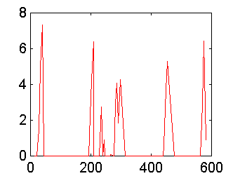
| 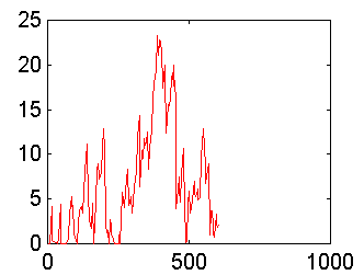
| 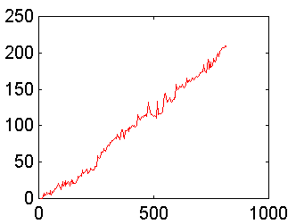
|
| Queue warte1
| Queue warte2
| Queue warte3
|
Each queue statistic considers all transactions moved through the respective queue.
Note that the relevant values for the plots are the queue entry time (x- axis) and
the waiting time (y- axix) of a transaction within the queue.
4. Evaluation
After finishing a simulation all kernel structures remain in memory an can
be inspected.
Additionally the kernel creates structures for visualisation the
queue utilisation. The name of the structure is a concatenation of
the respective queue name and the string stat.
To simulate the program simex1 the following commands have
to be entered at the Matlab prompt:
  datei='simex1.m'
  mainsimu
To show the server statistics for server1, enter servstat(server1).
To view the statistics of queue warte1, enter queustat(warte1).
To plot the queue utilisation of the queue warte1 enter
plot(warte1stat(:,1),warte1stat(:,2)), because warte1stat is a two
dimensional array, which contains tupel of the waiting time in a queue during
the current simulation time.
Alternatively the function plotqueu(warte1stat) can be used as a shortcut.
5. Restrictions and Conclusion
Because of the dynamic design of the interpreter the size of interpretable
GPSS programs is only restricted by local resources (memory).
A deviation to the real GPSS is that no labels can be interpreted. That means destinations
of jumps (transfer block) must be explicitly specified as line numbers (see examples).
Furthermore there is no error treatment implemented yet. All error messages
(e.g. wrong block name) come directly from Matlab and will not be evaluated by
the interpreter.
For future versions other statistical distributions for generating random numbers
(within generate, advance, transfer etc.- blocks) could be implemented.
Furthermore the set of defined blocks (in m- files) could be extended.
Wismar, 10. April 1998
u.dolinsky@iname.com