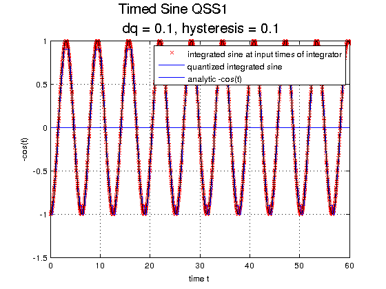
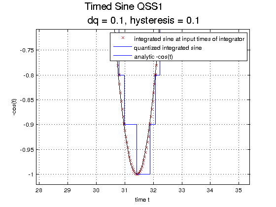
Plot for QSS1 Timed Sine Example

Plots the q-trajectory and X values of the integrated sine versus an analytically computed negative cosine function.

Contents

Call: plot_timed_sine_qss1(root_model,tstart,tend)

File: DEVSPATH/02-examples/discrete/sine-qss/plot_timed_sine_qss1.m

function plot_timed_sine_qss1(root_model,tstart,tend)

    % get the system parameters for figure titles
    dq = root_model.components.integrator1.sysparams.dq;
    epsilon = root_model.components.integrator1.sysparams.epsilon;

Plot via Manually Tracked States

    figure('name','Plot sine qss1 via manually tracked states','NumberTitle','off')
    hold on
    grid on
    plot(root_model.components.integrator1.s.traj(:,1),root_model.components.integrator1.s.traj(:,2),'rx')
    hold on
    grid on
    stairs(root_model.components.integrator1.s.qtraj(:,1),root_model.components.integrator1.s.qtraj(:,2))

    plot([tstart tend],[0 0])
    title(['Timed Sine QSS1 \newline dq = ',num2str(dq),', hysteresis = ',num2str(epsilon)],'FontSize',16);

    xlabel('time t');
    ylabel('-cos(t)');

    y=-cos(tstart:0.1:tend);
    hold on
    plot(tstart:0.1:tend,y,'k')
    legend  'integrated sine at input times of integrator' 'quantized integrated sine' 'analytic -cos(t)'
    hold off

Plot with the Observe Functionality

prerequisite: set observe_flag to 1 before simulation

    figure('name','Plot via observed states','NumberTitle','off');
    integrator1_t_values = [root_model.components.integrator1.observed{:,1}];
    integrator1_states = [root_model.components.integrator1.observed{:,2}];
    integrator1_X = [integrator1_states.X];
    integrator1_q = [integrator1_states.q];
    plot(integrator1_t_values,integrator1_X,'rx')
    hold on
    grid on
    stairs(integrator1_t_values,integrator1_q)

    plot([tstart tend],[0 0])
    title(['Timed Sine QSS1 \newline dq = ',num2str(dq),', hysteresis = ',num2str(epsilon)],'FontSize',16);

    xlabel('time t');
    ylabel('-cos(t)');

    y=-cos(tstart:0.1:tend);
    hold on
    plot(tstart:0.1:tend,y,'k')
    legend  'states s.X of integrator' 'quantized states s.q of integrator' 'analytic -cos(t)'
    hold off

end

---

DEVS Tbx Home      Examples      Modelbase           << Back

Published with MATLAB® R2014a